Figure 1. Flowchart Segment for data flow analysis.
| Home | Up | Questions? |
This thesis was presented to the Faculty of the Graduate School of
The University of Texas at Austin in Partial Fulfillment of the Requirements
for the Degree of Master of Arts.
This paper begins by presenting a problem common to computer software: correctness. Chapters 2,3, and 4 outline methods for preventing and detecting problems with the software before it is delivered to the end user. Chapters 5 thru 9 discuss in detail devices (known as debug tools) which can be used to isolate problems during execution which escaped detection during the coding stages. Finally, in chapters 10,11, and 12 a debug tool based upon ideas discussed in previous chapters is designed and implemented.
Our dependence on computers grows daily. Inventory control systems automatically reflect price changes, monitor sales, and reorder when stocks are reduced to a prescribed level. Airline reservations are maintained in real time by extensive computer networks. The design of spacecraft and even space travel itself would be impossible without computers. Soon computer systems may provide electronic funds transfer services for financial institutions.
The major expense in these (and most) computer systems now and even more so in the future is the cost of the software. Some researchers [30] believe that these costs might be as high as 90% of the total computer system by 1985.
This dependence on computer systems implies a need for correctness in these systems. Inventory control systems must correctly account for all sales. Airline reservations must not be lost or changed. The computation, monitoring, and correction of spacecraft orbits must be performed properly. Banks and their customers must have confidence that money will not disappear into the computer system.
Because of the high cost of software and the end-user's dependence on it, it is relevant to discuss methods which can be useful in the development of correct software. This development usually involves the following steps:
Throughout all of these steps correctness is an assumed attribute of the final product. It is not until the testing phase of development that the problem of establishing correctness becomes a reality.
What procedures can be used during the design and coding phases to increase the correctness of the final product? Program methodologies such as an adequate description of the problem to be solved, detailed design plans, coding standards, and code reviews provide a good environment for correct software production.
How is the correctness of software determined? The definition of correctness varies according to whose point of view is taken. The software is correct in the users' eyes if applications perform to their satisfaction. The quality assurance team agrees that the software is correct if their testing is successful. The programmer's ego may cause him to believe that his untried code is correct. The final answer to the question lies in actual experience with the system either by testing or by use at the hands of the end-user. There are, however, methods which can be employed before the experience stage to provide a higher level of confidence that the software is correct. These methods are collectively termed static analysis and will be discussed in more detail later.
It is inevitable that errors will be discovered during quality assurance testing and the use of any large, complex computer system. The problem then becomes one of locating the error in the source code in a cost effective manner. This is called dynamic analysis and is more commonly known as debugging.
This paper is concerned with the problems of producing correct software. More specifically it is concerned with some tools, in the form of computer programs, which can reduce the amount of effort necessary for the production of correct software. Techniques for developing and writing correct code are briefly presented. Methods (and tools) for determining the correctness of this software are discussed. Dynamic analysis, an important but often neglected area, is discussed in detail, including some examples of current work. A debug tool is proposed, implemented and evaluated.
The actual coding of a system should be delayed until a complete and detailed design has been produced. The urge to jump into the coding phase must be resisted. A careful design should uncover most of the problems which would otherwise be found during implementation. It is easier and cheaper to change the design than to change existing code.
Documentation is an important by-product of a detailed design effort. This documentation should include a description of all functional parts, the communication between these parts, and a description of the problem to be solved.
A structured design philosophy can be used to partition the problem into small well-defined, functional pieces. This partitioning must also specify the data and control flow between all of the individual pieces. After this point the coding becomes a mechanical process of converting the design specifications into a suitable programming language.
Even though the details of what to code are specified, the methods of how to generate this code need some guidelines. Coding standards such as establishing consistent naming conventions for variables, setting limits for the maximum complexity of modules, and prohibiting unclear and awkward coding constructions are useful. Module complexity is difficult to define, although the number of lines of code involved is a gross approximation. Code reviews are valuable but need to be handled carefully so as not to offend the author of the code. These reviews allow other staff members to become acquainted with the code and provide an opportunity for detecting errors and enforcing coding standards.
Testing is the process of gaining experience with the software, implicitly through day to day use or explicitly through use designed to exercise specific parts of the code. This testing may be at the individual module (subroutine) level or any combination of modules including the entire collection of modules known as the product. In any event the goal of this testing is to determine the quality (in terms of correctness) of the software.
Testing can be categorized into the following types. Each of these is discussed at greater length below. Subroutines PAGE1 and PAGE2 in appendix E will be used as examples in these discussions on testing. Both subroutines are supposed to compute the number of pages (PAGES) required to store a given number of words (WORDS). PSIZE is the page size.
Exhaustive testing is divided into two areas - processing all possible input data and executing all possible program paths. Testing which executes all possible program paths is certainly desirable but may not detect errors which are independent of the transfer of control characteristics of the program.
For example, subroutine PAGE1 has no flow of control statements. Hence all possible program paths can be exhaustively tested with a single set of input values. There is, however, an error in this routine. Whenever the number of words exactly fills some number of pages, the value computed will be one page too large.
Exhaustive data testing supplies all possible inputs to the software for processing. This is the only form of testing which can claim that a program is completely correct. Anything short of exhaustive data testing leaves open the possibility of errors in untested portions of the code. Exhaustive data testing is expensive in terms of machine and human resources. In general it is too expensive to be practical. It may be very difficult or even impossible to define all input combinations for complex systems. Even if the input can be generated there may be insufficient machine resources to perform the tests.
Consider a hardware multiplication unit which is designed to multiply two 27-bit integers in less than 100 microseconds [7]. Exhaustive data testing means that 2**54 different inputs must be tried. Ignoring the time to verify results, the multiplications alone would take more than 10,000 years. (An interesting fact derived from this result is that during the lifetime of this multiplication unit it will only be required to multiply a very small fraction of the numbers it was designed to process).
Program structured testing data is generated by dividing the input universe according to internal differences, that is according to the flow of control differences and the boundary conditions inside of the program. Detailed internal knowledge of the program structure is required to be able to produce data for this type of testing.
This example using PAGE2 tests the code which saves the
computation of PAGES if the current input values are identical
to the last input values. This section of code is not apparent
without inspection (or detailed documentation) of the code.
   WORDS PSIZE PAGES
    376   100    4
    521   100    6
    521   100    6
     49   100    1
    521   100    6
Data structured testing data is derived by partitioning the universe of inputs into classes according to external differences. Representatives from each class are then used in the testing process. In this case the partitioning is performed without regard to any data dependent processing inside of the program. Only the external characteristics of the data are considered.
This example tests PAGE2 for boundary conditions. Note that
PAGE1 fails with this test data.
               PAGE2   PAGE1
   WORDS PSIZE PAGES   PAGES
      0   100     0       1
      1   100     1       1
      2   100     1       1
     99   100     1       1
    100   100     1       2
    101   100     2       2
    498   100     5       5
    499   100     5       5
    500   100     5       6
    501   100     6       6
    502   100     6       6
Random testing inputs are chosen randomly from the universe of inputs. The only requirement for selection is membership in the input set. No consideration is given to internal or external characteristics of the data. Input for random testing is the easiest to provide.
This example tests PAGE2 with random input values.
   WORDS PSIZE PAGES
    372   100     4
     11   100     1
    186   100     2
    444   100     5
   6745   100    68
The most important (and most difficult) question to answer about testing is "How much testing is enough?". Since exhaustive testing is seldom practical, some technique must be employed to substantially reduce the number of inputs used for testing. This is the trade-off between the cost of complete testing vs. the cost of incorrect software. The end-user generally pays either way. He (often) pays real money and time for the development and testing of a software system. He pays again after the product is delivered if the vendor did a poor job or was pressured by the end-user to deliver the product too soon.
The testing process can be considered to be successful if the probability is low that the user will encounter an error. This implies that code which the user is expected to exercise often should be well tested while other code may receive little or no testing. This means that bugs may appear even after a program has been in use for many years. However this is the only practical solution to the extreme cost of exhaustive testing.
Static analysis or source code analysis is a semantic inspection of the source code for errors or questionable (but syntatically correct) constructions. A particular statement may be a legal statement in terms of the rules of the language but when taken within the context of other statements in the module or other related modules its meaning may be inconsistent with the intentions of the programmer. These are errors which can be detected mechanically and have been shown through experience to cause problems. This analysis is a planned attempt to discover problems before execution.
Static analysis is divided into the following areas which are discussed individually below.
Desk checking is the original method of source code analysis and is performed by humans with paper and pencil. The other types of static analysis are automated forms of desk checking, each specializing in a particular area.
Module analysis is limited to discovering simple programming errors in a single module or routine. These errors do not necessarily prevent the routine from functioning properly but rather indicate conditions which have a high probability of being incorrect and in need of attention by the programmer.
Some examples are:
Module interface analysis checks all routines in the system for inter-routine interface errors. More extensive checks for undefined variables can be made since information about all routines is available. Routine A may use (read) a variable which is an actual parameter for routine B expecting that B will return a value in that variable. The module interface checks can determine that routine B at least stores some value in the parameter used by A. If consistent naming conventions are used for variables in COMMON blocks, then the correct naming and alignment of such variables can be verified. Also conflicts between the number, size, and type of formal and actual parameters can be reported.
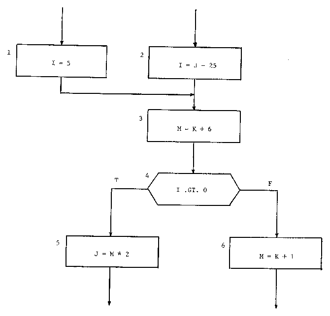
Data flow analysis is a study of the way data is used within a program. In general data is input to a program, the program performs some computation using the input data, and finally produces some output data. The computation process within the program is the area of interest in data flow analysis. A general assumption is made that for a given computation input was derived from the result of a past computation and the result of the given computation will be used as input for a future computation. A data flow anomaly occurs if this pattern is violated. For example:
          .
          .
          .
          X = 3.5 + Y
          X = Z*R
          .
          .
          .
The result of the first computation is never used since it is destroyed by the second computation. If this is really what the programmer intended, then the first computation can be deleted without changing the output of the program. This is an obvious and trivial example. In practice these two statements would be separated by other statements or even be in different routines thereby complicating the analysis.
A data flow anomaly is a potential problem only if it can be executed. Consider the flowchart segment shown in Figure 1.
Figure 1. Flowchart Segment for data flow analysis.
The detection of data flow anomalies requires that all routines in the system be involved in the analysis. First all anomalies are located. Then, for each anomaly, a path containing the anomaly is isolated. Finally a determination of whether or not the path is executable is attempted. If the path cannot be executed, then it is ignored.
Proofs of correctness attempt to prove by formal mathematical techniques that a program has been coded correctly, that is that the code will behave according to the specifications for the solution. An example is proof of correctness by inductive assertions. In this method assertions about the program state are inserted by the programmer or prover after each line of source code. The correctness is proved by demonstrating that each of these assertions is true whenever the program is in that state, assuming that at each previous step a true assertion was encountered.
A second method is proof by partitioned analysis of the cases to be covered. This is a code analysis rather than a programming technique like proof by inductive assertions. The proof consists of dividing the input data into mutually exclusive classes and analyzing each class for correctness.
Correctness may be difficult or impossible to determine in many cases. Sites [34] has attempted to address some of these areas by considering a proof of clean termination in lieu of a proof of correctness. A proof of clean termination does not guarantee correct output but it does guarantee that the program will not be caught in an infinite loop or terminate abnormally due to execution errors such as address out-of-range or accumulator overflow.
The use of static analysis techniques allows some common programming errors to be located in the source code before execution. It is important to note that locating the error in the source code using static analysis is far superior to waiting until execution and working backward from the incorrect output to the source code. Except for desk checking, these methods are automated and may require little investment of time from the programmer. Since execution is not required, it is not necessary to prepare input data. The checkout (debug) phase of software development receives a product with fewer bugs. Hence checkout time is reduced.
Desk checking is slow and susceptible to human error. The utilities which perform the static analysis are often expensive to execute because of the large amounts of computation involved in analyzing the source code. These analysis utilities are language dependent, at least at the syntax level, and are not generally applicable to assembly language. Simple logic or keypunch errors such as M=M+1 instead of M=M+2 cannot be detected. Only a few static analysis utilities are currently available.
Even if a proof of correctness for a program is true, there is still the possibility that the program will produce incorrect results when it is executed. The proof operates on the source code and does not consider the details of converting the source code to machine code and executing the program on a given hardware configuration. Details of computation such as accumulator overflow and the mechanics of passing parameters to subroutines may cause a program to malfunction even though it was proved to be correct.
In general, programmers do not write code in a style which is compatible with proof of correctness techniques. Numerous programming "tricks" or efficient coding constructions can be very difficult to analyze during the proof. Prokop [29] believes that new programming philosophies will need to be developed before proof of correctness techniques can be generally useful. The programmer must be concerned with producing code which correctly implements the program solution and in addition is not confusing to the program prover. These new coding techniques will probably sacrifice execution efficiency for provability.
Many existing programming languages are ill-suited to formal proof methodologies. Two new programming languages, EUCLID [25, 26] and GYPSY [1], have been specifically designed to be verified by either manual or automatic formal proof techniques. These languages are based upon PASCAL and are not necessarily general-purpose. Also they may be somewhat difficult to use and the object code produced by the compilers may not be the most efficient but that is probably the price to be paid to verify programs at the source code level.
Dynamic analysis, more commonly known as debugging, is employed to isolate errors in the program which cause incorrect results to be observed during execution. All problems in the software which could not be or were not detected by other means must be resolved by dynamic analysis. Testing will show that a program is incorrect but will not locate the source code which caused the error. Since most programmers produce bugs, debugging is expected during checkout but the details cannot be planned since it is not known what errors will occur.
Dynamic analysis techniques are divided into the following categories and discussed below.
Desk checking is the oldest type of dynamic analysis. The most basic form requires that the programmer simulate the computer with paper and pencil using the source code and the incorrect results. To some degree desk checking is involved in all types of dynamic analysis.
A post mortem dump is a display of the contents of memory at the time that the program terminated execution. Errors can often be found by comparing assumed values of certain memory locations with actual values from the dump. In general the dump may be the only aid provided by the operating system to help locate an error.
A debug tool is a device which is used to reduce the number of aspects of a program's behavior which are misunderstood or poorly understood by its programmer. Implicit in this definition is the fact that a debug tool does not locate errors in the source code. It only serves to provide information about the execution of the program which would otherwise be difficult or impossible to obtain. This information is then used as an aid to the programmer in his search for the cause of the error in the source code.
Debug tools are implemented either as modifications to the malfunctioning program or as a standalone utility which can monitor the execution of the program. Program modification by the user usually takes the form of inserting print statements to display the contents of various variables and to trace the paths taken through specified segments of the code during execution.
Program modification by a utility program may be performed by a precompiler which modifies and adds code according to user directives. Features of such a precompiler include the ability to trace subroutine calls, to display variables, and to perform execution-time verification of program states. This last feature may require that the programmer add assert statements (comment cards) to the program describing the values and relationships which the programmer believes certain variables should have. The precompiler reads the assert statements and generates code to check for these values during execution.
Another form of debug utility is a debug compiler (also known as a checkout compiler) which is used during initial development of code. These compilers require more memory and more execution time but they provide the additional services of some of the static analysis utilities discussed previously. When the code is finally debugged it is compiled on a standard compiler which is more efficient and produces object code without debug prints and traces.
A monitor utility operates on the object code either in relocatable or absolute format. For this reason it is language independent except perhaps for the user/utility interface which will be discussed later. The monitor utility concept requires fewer (perhaps no) program modifications when compared with other forms of debug tools. The monitor provides much greater control over program execution with such features as breakpoints and interrupts on references to specified variables. Moreover this control over execution can be performed in real time if interactive access is provided. In essence the monitor utility is a virtual machine supplying an execution environment with user control which is transparent to the program being debugged.
Desk checking is slow and subject to the same human errors that caused the bug. In addition the incorrect output is often insufficient to locate the source code that caused the error. Post mortem dumps provide no execution history, only a final snapshot of memory. Depending upon the size of the program, the dump may produce a considerable amount of output, usually in octal or hexadecimal, which must be decoded. Debug features built into the program by the programmer are usually an afterthought and not general enough to be useful for fixing other bugs. These built-in features can have bugs when they are added and cause bugs when they are removed. Program modification can cause the manifestations of the bug to change or disappear altogether. Also it is just plain inconvenient to modify the program to insert debug statements.
It is often desirable to leave built-in debug features in the program to help solve future problems. The debug features can be incorporated into the program so that they are normally inoperative. By changing the value of a switch, the debug code can be invoked. Multiple values for the switch or multiple switches can enable selected portions of the debug code instead of all of it at once. The disadvantage of this technique is that the debug code may require considerable memory even when it is not used.
Program modification by a utility overcomes many of the objections to user modification of the program. However the utility may not be flexible enough to display the kinds of data necessary to find the bug. Also the utility cannot provide much control over the program's execution. Since the utility must read the source code it is language dependent.
A monitor utility provides considerable control but the user is required to learn the language of the utility in order to be able to communicate with it. (This is a problem with all utilities). Because the utility deals with the program as it is represented by machine code, the user may need to know more about the details of the operating system, compiler, assembly language, etc. than would otherwise be necessary. For example, the machine code generated by the compiler for a given source statement may be intermixed with machine code for other source statements.
Debug tools may vary widely in the capabilities and services they provide for the user.
The following common debug features are informally described for the benefit of future discussion.
Breakpoint - the ability of the debug tool to interrupt the execution of the job at a user-specified location. Control is then passed to the user for additional directives. One of these directives may be to restart the job from the point of interruption.
Memory and register dumps - the ability to print the contents of selected memory locations including the program's registers. The items to be dumped may be printed in various formats including octal, decimal, and character.
Memory and register modification - this feature allows the user to change the contents of selected memory locations and registers. Modifications may be entered as source statements, numeric, or character values.
Monitor memory locations - the debug tool monitors every read and/or write for specified memory locations. A breakpoint can be generated if a certain value (including any value) is stored into (or read from) one of the specified locations.
Trace - a feature which prints the "instructions" being executed. The output format might be machine code, assembly language mnemonics, or higher level source language statements. The values of any variables or registers involved may also be printed.
Reverse execution - this provides the ability to execute the program in a backwards direction from some point of interruption. The distance one may travel backward may vary, depending upon the implementation, from only a few instructions to all instructions involved.
Checkpoint/restart - a checkpoint saves the current state of the program. At a later time the program can be restarted from this "saved state". If appropriate checkpoints are taken, this feature can simulate reverse execution by restarting a checkpoint taken prior to the error.
Branch history - this is a record of every (or the last n) transfer of control changes within the program. This information may be used for manual reverse execution.
Symbolic addressing - many debug features require the user to specify memory locations to the debug tool. Symbolic addressing allows the user to identify these memory locations by the same names (symbols) which were used in the source language. This requires the debug tool to have a symbol table for use in converting the symbols to actual addresses. The symbol table may be constructed from compiler and loader output either by the debug tool or a separate utility program.
Execution statistics - depending upon the implementation scheme, the debug tool may be able to collect information about what part of the code is being executed by the CPU most often and how many and what kind of requests are made to the operating system, e.g., I/O requests.
Instruction step - this feature initiated from a point of interruption (e.g., breakpoint) allows n (usually small) words of instructions to be executed before control is returned to the user. The n instructions executed may or may not be traced.
Snapshot dumps - these dumps are generated automatically by the debug tool as the program executes. Their content and frequency are specified before execution by the user.
Although program modification by the user is considered to be a valid debug tool, this paper will concentrate on debug tools implemented as utility programs. Of all the possible utility programs those which can be classified as monitor utilities are the most interesting because they provide the most control over program execution.
First, all programmers produce bugs. As previously discussed, techniques exist for analyzing source code for potential bugs but they cannot guarantee that the code produced is free from bugs. Thus debugging is inevitable. In fact debugging accounts for more than 50% of programmer time [35]. Debugging is the most tiring, expensive, and unpredictable phase of software development [11]. Debug tools can significantly reduce the time and effort required to locate a bug by providing dynamic displays of program states and by providing control over program execution. The operating system usually provides no more than a post mortem dump. Little attention is given to debugging in texts and universities. It is reasonable to devote time and effort toward the production of sophisticated debug tools to make the debug phase of software development easier and faster for the programmer.
Consider the following situation: The output from a program is correct but it costs $1000 for a single run. This is not an unusual problem. Several possibilities exist for explaining the high cost of running the program.
While not generally designed for performance measurement applications, debug tools can help determine some of the causes of poor performance. CPU execution statistics (if provided by the debug tool) can isolate areas of the code which are executed frequently. Visual inspection of the code is then necessary to determine if a problem exists. In the buffer manager example above, traces and dumps triggered by execution of the code performing the I/O can be used to reveal a malfunction.
Implementation options include:
In general a debug tool will not strictly adhere to a single implementation scheme but rather will use a combination of methods by implementing a particular debug feature by using the most effective method.
Modification of source code by a precompiler causes statements in the source language to be inserted at appropriate locations to provide dynamic displays of program states and trace information. Once the source code is compiled, the debug commands are frozen. Any change in the debug command sequence requires re-precompilation and re-compilation. The problem of trapping references to a specific memory location is handled symbolically and not by actual address. This means that assembly language code or compiler-level source code could reference the memory location in question by a clever addressing technique which could not be detected by the debug tool. This is the well known alias problem with variable names.
Modification of object code requires a monitor utility at execution time instead of a precompiler. The monitor modifies and/or replaces certain machine instructions to gain control at times indicated by user directives. If interactive access is provided, this implementation method allows real-time decisions to be made about what action to take next. In the precompiler mode all such decisions must be made in advance at precompile time. Using this method alone it is not possible to trap references to a specified memory location without the help of hardware.
In certain situations the debug tool can be implemented as a standalone hardware device capable of monitoring the executing program. An example is a device which can determine which part of the program uses most of the CPU resources. More common is the use of certain existing hardware features which allow the debug tool to detect situations which would be difficult to determine otherwise. For example, a machine with memory parity bits could have the parity bit toggled by software in a memory location in such a way as to force an interrupt into the debug tool if that memory location was referenced. Thus to trap memory references the debug tool sets the appropriate parity bit and waits for the interrupt.
Software interpretation of the machine instructions by the debug tool is often necessary when the hardware does not support features to allow a debug feature to be implemented otherwise. The example of trapping specific memory references can be done easily through interpretation. The major disadvantage in this method is its increased execution cost.
User access to the debug tool can be through batch or interactive methods. The one advantage that batch provides over interactive is the large amount of output that is possible in this mode. Interactive mode may allow large output files to be spooled to a printer thus overcoming this obstacle. The breakpoint feature of a debug tool is highly oriented toward interactive use. The decision of what to do next can be made in real time based upon output from previous commands. Studies by several groups [31, 11, 8] have shown that programmer productivity is higher when interactive access methods are used.
The user must provide directive (commands) to the debug tool to tell it what to do. These directives should be flexible, brief, and easy to learn. It should not be necessary for the user to spend a lot of time and effort learning a lengthy, complex language to be able to use the debug tool. The commands must name entities within the program which are of interest to the programmer. These entities should be described to the debug tool in terms and concepts of the source program.
Output from the debug tool should be easy to read and in terms of data formats consistent with the source program.
All of this communication requires that the debug tool have access to information such as names, locations, and types of subroutines and variables within the source program. This data is generally available from load maps and compiler listings. Either manual or automated methods can be used to format this data into a symbol table for use by the debug tool.
Current work was examined for certain attributes and will be presented in the following format:
In the discussions that follow, user program, uprog, and program to be debugged all have the same meaning.
A debug tool named HOPE (Helper for Observation of Program Execution) was developed for a specific environment but is general enough to be useful for numerous other applications. The Control Data 6000 series computer and the NOS 2.1 operating system provide the basic operating environment for HOPE. The programs requiring debugging aids are production and development programs written in FORTRAN and COMPASS (the CDC assembly language) consisting of several hundred subroutines and numerous overlays. Although HOPE allows some symbolic input, the output is at the assembly language level. Thus the user must have a good working knowledge of compiler and assembler listings and loader maps. Policy restrictions for the computer prohibited any modifications to the operating system and permitted only remote access through RJE and TTY terminals.
First, because good debug tools are extremely useful devices. That is the major point of this paper. And second, because the vendor (CDC) does not supply any such tools for the environment previously described. It should be pointed out however that the operating system comes with a very powerful debug facility which is only accessible from the on-site console. Although this debug facility provides numerous features, it is deficient in some areas. For example it is not possible to trap references to memory locations.
The discussion in this section includes batch and interactive (TTY) processing. Explicit references to either type will be made only when the processing is different. The phrase "return control to the user" means read the next command from an interactive device or from the batch input card.
Non-symbolic operands are limited to octal numbers to be consistent with the operating system software. The compilers, loaders, and assembler all display addresses in terms of octal numbers.
Relationship is denoted by <rel>. Address expression is denoted by <ae>. Address range is denoted by <rg>.
<octal digit> ::= 0 | 1 | 2 | 3 | 4 | 5 | 6 | 7
<decimal digit> ::= <octal digit> | 8 | 9
<octal number> ::= <octal digit> | <octal digit><octal number>
<n> ::= <decimal digit> | <decimal digit><n>
<register> ::= A0 | A1 | A2 | A3 | A4 | A5 | A6 | A7 |
X0 | X1 | X2 | X3 | X4 | X5 | X6 | X7 |
P | B1 | B2 | B3 | B4 | B5 | B6 | B7
<rel> ::= NE | EQ | LT | GT | LE | GE
<operator> ::= + | -
<symbol> ::= a string of up to seven alphanumeric
characters, the first is alphabetic.
A member of the set of symbols in the
symbol table. <symbol> <register> = 0.
<operand> ::= <symbol> | <octal number>
<ae> ::= <operand> | <operand><operator><ae>
<rg> ::= <ae> | <ae>;<ae>
<blank> ::= one or more blank characters
<value> ::= <octal number> | <octal number><blank><value>
{ } ::= optional syntax delimiters. The item(s) may or may not be used.
<at cmd> ::= DMP | BKP | DMP{,}<rg>
<if cmd> ::= <at cmd> | PRINT
<if action> ::= <if cmd> | <if cmd>/<if action>
<at action> ::= <at cmd> | <at cmd>/<at action>
Within <if action> and <at action> PRINT, DMP, and BKP may occur only once but DMP<rg> may occur multiple times. The maximum number of occurrences is described under RESTRICTIONS and LIMITATIONS.
DMP
DMP{,}<rg>
RESET{,}<register>=<value>
RESET{,}<ae>=<value>
STEP{,<n>}
STEP {<n>}
LIST
HALT
CLEAR
CLEAR{,}<rg>
GO
ENTER{,}<symbol>=<ae>
BKP{,}<rg>{,<n>}
TRACE{,}<rg>{,<n>}
IF{,}<ae> IS READ,<if action>
IF{,}<ae> IS WRITTEN,<if action>
IF{,}<ae>.<rel>.<value>,<if action>
AT{,}<ae>,<at action>
AT{,}<ae>,IF{,}<ae>.<rel>.<value>,<if action>
DMP provides the ability to display registers and contents of memory locations. DMP with no arguments displays the location counter, field length, and CPU registers. If arguments are present the contents of memory locations specified in <rg> are displayed in octal and character formats with the address of each location. See Figures 2 and 3 for sample output. Control is returned to the user after execution of DMP. Examples:
DMP
D,37
DMP TEST;TEST+16
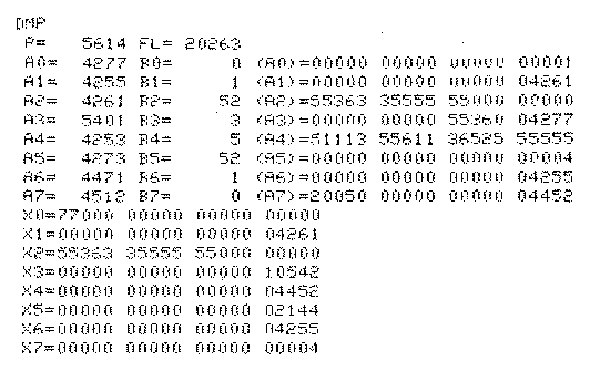
Figure 2. Example of Exchange Package Dump
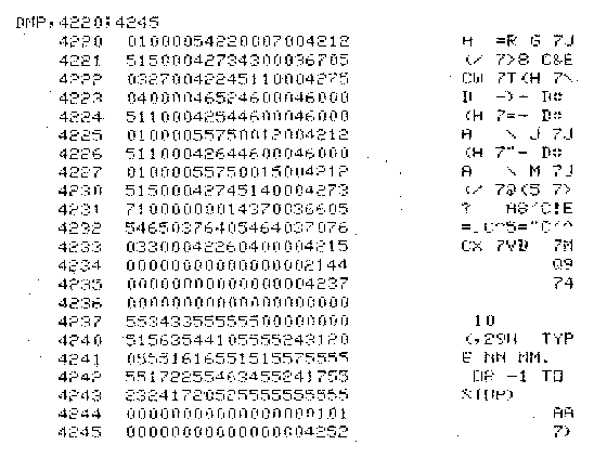
Figure 3. Example of Memory Dump
RESET allows the contents of registers and memory locations to be changed. Since symbols and registers cannot have the same name, no ambiguity arises in distinguishing between them. Blanks are allowed in <value> for readability. Control is returned to the user after execution of RESET. Examples:
RESET,X6 = 230
R COUNTER=24
R,TEST+6 = 51300 06345 10733 46000
STEP allows a specified number of words of instructions to be executed before control is returned to the user. If <n> is absent, <n>=1 is used. For each instruction, the memory location, the instruction mnemonic, and the value of the resultant register are printed. See Figure 4 for sample output. Examples:
S
STEP,6
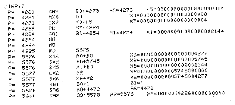
Figure 4. Example of Step and Trace output.
LIST displays all pending deferred commands which have been entered by the user. Control is returned to the user after execution of LIST. See Figure 5 for sample output. Example:
LIST
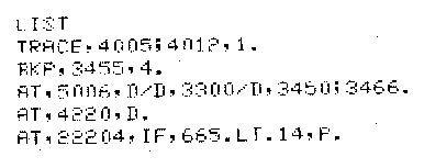
Figure 5. Example of List output.
HALT terminates the execution of the debug tool (as well as the execution of the program being debugged). Control is passed to the operating system for execution of the next JCL statement after entering HALT. Examples:
H
HALT
CLEAR deletes pending deferred commands. If <rg> is specified, all pending commands which are bounded by <rg> are deleted. If <rg> is absent, all pending commands are deleted. Control is returned to the user after execution of CLEAR. Examples:
C
CLEAR,TEST+2;TEST+30
C 376
GO transfers control (the CPU) from the debug tool to the program being debugged. That is it restarts (or starts) execution of the program being debugged from the point of last interruption. Control may or may not be returned to the user depending upon the presence of any deferred commands. Example:
GO
ENTER allows symbols to be entered into the symbol table. Control is returned to the user after execution of ENTER. Examples:
ENTER,CTYPE = 3457
E LEVEL = TEST + 26
BKP (breakpoint) allows the user to specify the location(s) at which execution of the program being debugged is to be interrupted. A breakpoint is set in each location specified in <rg>. If <n> is specified, the interrupt is performed only after the breakpoint has been encountered <n> times. If <n> is absent, <n>=1 is used. When the breakpoint has been encountered <n> times, control is returned to the user.
BKP is a deferred action command. This means that the command is stored in a table until the program being debugged is in execution and the conditions specified by the user are satisfied. At this time the command is executed. Since the debug tool stores a jump at <rg> to gain control from the user program, this location(s) must not be changed during execution.
B,24673
BKP TEST+200,6
TRACE prints the location, instruction mnemonic, and resultant register when the instructions bounded by locations in <rg> are executed. The output for TRACE is identical to the output for STEP. The TRACE output is provided <n> times for a given <rg>. If <n> is not specified, <n>=1 is used. TRACE is a deferred action command. Examples:
T,TEST+17,4
TRACE TEST+3;TEST+7
IF allows a memory location to be monitored during execution for any read, any write, or any write which satisfies a relationship to a given value. This is a deferred action command and the action performed depends upon the commands specified by the user in <if action>.
PRINT displays the address of the instruction accessing <ae> and the contents (after execution of the instruction) of <ae>.
DMP displays the values of all registers and memory locations as described previously.
BKP returns control to the user. If BKP is specified, it is executed last.
The IF command stays in effect until it is deleted by a CLEAR command. Examples:
IF,TEST .GT. 0,P/D TEST;TEST+4/D TEST+30;TEST+41
I LEVEL IS READ,BKP
IF 36537 IS WRITTEN,PRINT/BKP
AT specifies that the execution of the program being debugged is to be interrupted when instructions at location <ae> are executed. The action(s) to be taken after interruption is specified by the user in the <at action> clause. Items in <at action> are described under the IF command. AT is designed to provide snapshots of memory and registers during execution. AT is a deferred action command and is in effect until cancelled by CLEAR. Examples:
AT TEST+5 , DMP TEST+100;TEST+110
A,37521,BKP is equivalent to BKP,37521
AT DRIVER+17,D/D 101/D 267/D 5743
AT..IF - this command is more efficient than IF alone. The IF part of the command is only executed when the AT is satisfied as described above. This is a deferred action command and remains in effect until deleted by CLEAR. Examples:
AT,DRIVER+27,IF SIZE.EQ.37,BKP
A TEST,IF 3462 .NE. 7777,P/D,306;310
AT DRIVER+7, IF FLAG .NE. 0,D/P/B
Note about IF and AT..IF - the IF command requires full interpretation of the machine instructions and therefore causes a high CPU overhead. The AT..IF command executes at normal CPU speed until the location specified by <ae> is reached. At that point the IF part of the command is evaluated and execution continues or the <if action> clause is executed. If it is only necessary to evaluate the IF command at a few discrete locations , then the AT..IF command should be used. However if it is necessary to monitor all references to <ae>, then IF must be used.
As the debug tool controls the execution of the user program certain conventions must be followed so that the debug tool's presence remains transparent to the user program.
The transparent mode of operation is the principal interface method. In this mode, the debug tool loads the program to be debugged into memory just as if the operating system had done it. This is a trivial operation because the user program is required to be in absolute (already relocated) format and the debug tool simply transfers uprog from disk to the appropriate place in memory. Figure 6 shows a memory layout for the debug tool and uprog in this mode. Before passing control (the CPU) to the user program, the debug tool interrogates the user for debug directives.
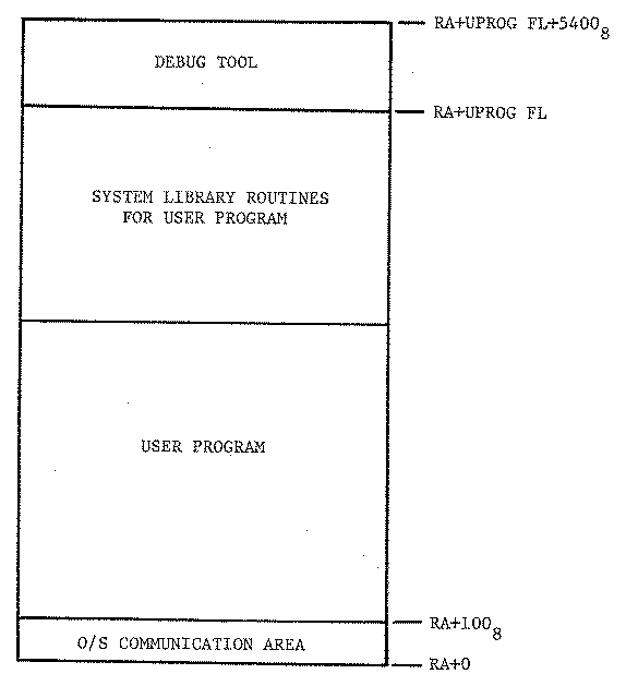
Figure 6. Memory layout for transparent mode.
If any control card parameters are required by uprog, they are entered on the HOPE control card exactly as they would be on the control card used to execute uprog. HOPE does not modify the memory reserved for these parameters. Thus uprog can process them when it receives the CPU.
HOPE provides a transparent execution environment for uprog while maintaining control over the execution. No modifications to uprog are necessary to debug in this mode. HOPE however must be configured with sufficient memory to allow uprog to be loaded. The procedure for doing this will be discussed later.
Certain situations arise where uprog needs memory which is not allocated at the time the loader converts from relocatable to absolute code. An example is a COBOL program which obtains and releases memory for buffers during execution when files are opened and closed. This memory management is performed by the operating system library routines and is not under user control. In transparent mode, uprog is unaware of HOPE's existence and will allocate or deallocate memory which is occupied by HOPE.
To overcome this problem, the semi-transparent mode of operation was devised. Both uprog and HOPE are in relocatable format. The two relocatables are combined by the user (see appendix A for sample control cards) and loaded into memory by the operating system. Figure 7 provides a memory layout for semi-transparent mode. In order for the debug tool to ever receive control, the user must insert a CALL HOPE source statement in uprog. When this statement is executed the debugging session begins as if transparent mode were being used.
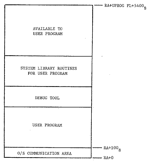
Figure 7. Memory layout for semi-transparent mode.
INPUT - this file contains all commands. The format is card image. INPUT is also the name of the interactive input device for interactive mode.
OUTPUT - this file contains all output generated as a result of executing commands including diagnostic and informative messages printed by HOPE. The format is standard printer line image. OUTPUT is also the name of the interactive output device for interactive mode.
UPROG - this file contains the program to be debugged when using transparent mode. Its format is that of an absolute program file created by the loader.
SYMTAB - this file contains the optional symbol table. It is read into memory as part of the initialization process of HOPE. The file consists of one-word entries terminated by a full zero word. The entry format is 42/<symbol>,18/<value> where <symbol> is left-justified, binary zero filled display code and <value> is the integer value of the symbol.
Normal operating system procedures would allow these file names to be changed at execute time by appropriate control card parameters. Since the control card parameters used with HOPE are intended for uprog, HOPE does not (and cannot) process them. Thus these names can be changed only by source code modification to the debug tool.
All programs communicate with the operating system by means of an RA+1 request. RA is address zero of the user program; hence RA+1 is the second word of the program. The operating system monitor constantly samples RA+1 of the program in memory which has the CPU. When RA+1 becomes non-zero, the monitor interprets the non-zero value as a request for some service (e.g., I/O, time of day, tape request). The CPU may be taken away from the program until the request is completed by the operating system if a certain bit is set in the RA+1 request. Otherwise the program keeps the CPU and must perform the completion check itself.
The debug tool does not interfere with this communication between the user program and the operating system. There are however two situations which the debug tool must be aware of. First, it is possible for the debug tool to receive the CPU when RA+1 is non-zero. In this case the debug tool must wait until the operating system monitor accepts the request before proceeding. Also the debug tool does not give the CPU to the user program if RA+1 is non-zero. Second, before the debug tool flushes the output buffer for the user program, it must first check to insure that the previous I/O operation has been completed.
HOPE was implemented as a monitor utility. Except for the addition of one source statement in semi-transparent mode, no modifications to the program being debugged are required. HOPE was written primarily in COMPASS (the CDC assembly language) with some FORTRAN for a total of 6300 lines of code. Memory requirements are 5400 (octal) words.
The language (commands) recognized by the debug tool is defined through the use of Floyd-Evans productions [9]. Appendix B contains the language definition written in these productions. A precompiler reads the productions and produces an assembly language table for inclusion with the other debug tool routines. A command parser reads each command and breaks it down into syntactic units. (A syntactic unit is a string of alphanumeric characters or a single special character). These syntactic units are matched with entries in the Floyd-Evans production table to determine if the command is valid. Data contained in each production table entry tells the parser where the next syntactic units are and how many should be matched at a time.
Messages produced by the debug tool are listed in alphabetical order. An explanation is also provided for each message. Command fatal (CF) messages cause the entire command to be rejected. Job fatal (JF) messages cause the job to be terminated abnormally. Messages which are applicable to transparent mode only are indicated by (T). Those messages which are applicable only to semi-transparent mode are indicated by (ST). Lack of a T or ST designation means that the message can be received in either mode.
The execution of deferred action commands must wait until the program being debugged reaches certain user-defined conditions. Thus these commands are entered into the deferred command table (DCT) to be executed at a later time. Each deferred action command exists in the DCT as one or more records. Each record is the same size and contains a record type identifier. A single command, depending upon its complexity, may require multiple records in the DCT chained together in a linked list structure. The first record of the chain contains the breakpoint address and the word of instructions which were replaced by the breakpoint. The breakpoint itself contains the address of this first record so the debug tool can execute the appropriate command when it receives control. Examples are TRACE, BKP, AT, and IF.
BKP - the breakpoint routine replaces the word of instructions at the breakpoint address with a word containing a return jump to the breakpoint processor and the address of the breakpoint record in the deferred command table. The replaced instructions and the breakpoint count are saved in the breakpoint record. When the breakpoint processor is called (as a result of executing the return jump at the breakpoint address) the registers are saved and the breakpoint count is decremented. If the count is exhausted, control is passed to the user. Otherwise the registers are restored, the saved instructions are executed remotely and control is returned to the user program. Remote execution is performed by storing the saved instructions in the first word of a two word array, storing an unconditional branch to the breakpoint address+1 in the second word of the array, and transferring control to the saved instructions. Control is returned to the user program by executing a branch instruction (one of the saved instructions) or executing all saved instructions and falling through to the second word of the array.
TRACE - the trace feature uses a breakpoint to get control when the first word of the trace range is executed. The registers are saved and interpretation of the instructions begins and continues until control is transferred out of the trace range. In trace mode during interpretation, each instruction, its address, and the value of the resultant register is printed. When control is transferred out of the trace range, interpretation stops and the trace count is decremented. If the trace count is not exhausted, the trace breakpoint is reset. Finally the registers are restored and control is returned to the user program.
STEP - interpretation begins from the point of interruption and continues for the number of words of instructions specified as the step count. During interpretation the instruction, its address, and the resultant register are printed just as in TRACE mode. Control is returned to the user when the step count is exhausted.
DMP - the values of all registers are saved whenever control is passed from the user program to the debug tool. Information from this save area is used to produce the output for this command.
RESET - the first symbol in the address expression is compared with the register names. If it is a register, then the appropriate value in the user program's register save area (exchange package) is changed, otherwise the appropriate memory location is changed.
GO - this command returns control to the user program. Control may be transferred by restoring the registers and returning the real CPU to the user program or by starting (or restarting) the interpreter. The presence of any IF commands in the deferred command table causes the interpreter to be used.
ENTER - the input symbol is examined to be sure that it begins with an alpha character and is no longer than seven characters. Then a search is made for it in the symbol table to prevent duplicates. Appropriate diagnostic messages are printed for errors.
IF - the IF command requires interpretation of the user program. A table of addresses which are to be monitored is examined for each memory reference, excluding reading memory for instructions. If a match is found, then the table of addresses contains the address of a record (or records) in the deferred command table which defines what action(s) to take. Interpretation is resumed after processing the action record(s).
The algorithm (exhaustive table search for every memory reference) for determining if a memory reference is for an address in the table is suitable only for a small number of entries in the address table. Other algorithms which search the table only if the address in question has a very high probability of being in the table could be implemented if use of this feature required the monitoring of numerous locations.
AT - this command uses a breakpoint to transfer control to the AT processor. The breakpoint also contains the address of a record (or records) in the deferred command table which defines the action(s) to be performed. As with IF, execution resumes after the action(s) has been carried out.
AT..IF - this command allows the user program to be executed at normal speed (rather than be interpreted) and still take advantage of the power of IF. The IF part of the command is evaluated when the AT breakpoint is reached.
LIST - each deferred command is represented by one or more records in the deferred command table. Each record contains a type field which is used by LIST to determine which commands are in the table.
CLEAR - each deferred command record contains the address it is associated with in the user program. These addresses are used by CLEAR to determine if a record falls within the CLEAR range and therefore should be deleted. CLEAR must also replace all instructions which were displaced as a result of breakpoints.
HALT - this command closes the output file for the debug tool and the user program (if it has a file named OUTPUT). Then it terminates execution of the debug tool and returns control to the operating system.
Items 1,2,3, and 4 may easily be changed by re-definition of the symbol which is used to specify the size of the appropriate buffer or table. Appendix C contains a list of such symbols.
The NOS operating system provides a sub-tasking facility called a sub-control point (SCP). A control point is a software-defined resource which a job possesses if and only if it occupies central memory. A job (job A) at a control point can use the SCP facility to create one or more tasks (job B) which execute at sub-control points under control of the initiating program (job A). Job B executes exactly as though it were at a control point. It has its own memory bounds and registers. Job A defines the memory bounds, has access to all memory for job B, and transfers the CPU to job B. Job A receives the CPU (from job B) under the following circumstances:
This is an excellent environment for a debug tool (job A) to control the execution of a malfunctioning program (job B). See Figure 8 for a memory layout of such a job which has one sub-control point. The problems discussed earlier of memory allocation by the user program (semi-transparent mode) and configuration of a proper "hole" for transparent mode disappear when using a sub-control point. The difficulty with SCP mode is that job A intercepts all RA+1 requests from job B. This means that the RA+1 request must either be processed by job A or passed on to the operating system. In any case the parameters (addresses) used in the RA+1 request are relative to job B but if they are passed on to the operating system they must be relative to job A. Thus job A must relocate all such addresses, pass the request to the operating system as if it were making the request, un-relocate the addresses, and return the CPU the job B. Thus the debug tool would be required to simulate the operating system for the user program. The decision not to use the SCP feature in the debug tool was made for this reason.
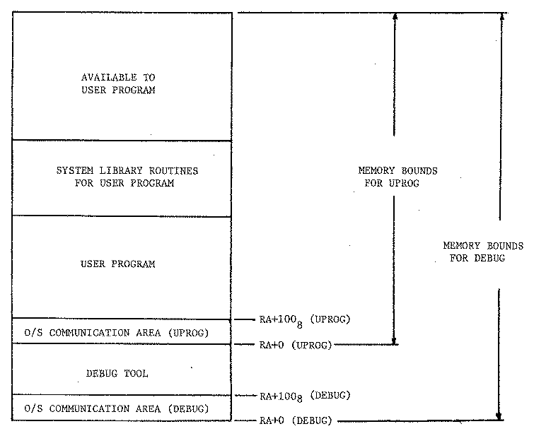
Figure 8. Memory layout for sub-control point (SCP) mode.
Virtual storage exists when the logical address space is different from the physical address space for some real device. A virtual machine is a generalization of virtual storage. It is a computing system in which the instructions issued by a program may be different from those actually executed by the hardware [28].
Goldberg [12] defines two types of maps based upon the mapping of real resources to virtual resources in a virtual machine. The p-map is an intra-level map and is software visible. It maps process names to resource names. The f-map is an inter-level map and is software invisible. It maps virtual resource names to real resource names.
In general a debug tool implemented as a monitor utility provides a virtual machine environment for the program being debugged. The current implementation of HOPE follows Goldberg's p-map. An implementation using the SCP feature would follow the f-map.
Figure 9 is an example of monitoring all RA+1 requests for a FORTRAN program named AUDIT. The debug tool was requested to print any value which was stored in address 1 (RA+1). Such values contain the name of the PP program being called in bits 59-41. Bit 39 is the auto-recall bit and bits 17-0 contain the memory address of input/output data. In the case of the PP program CIO, bits 17-0 contain the address of a file environment table (FET). The FET contains the file name, a function code, and buffer pointers for I/O operations [39].

Figure 9. Example of monitoring all RA+1 requests for a program.
All I/O requests performed with a given FET can be displayed by the technique shown in Figure 10. (This is the same program that was used for Figure 9). In this example the debug tool dumped the FET only when RA+1 had a CIO request for the FET at address 5414.

Figure 10. Example of monitoring all I/O requests for a given File Environment Table (FET).
Desk checking a piece of code is a good technique for finding errors. However, the same incorrect assumption made during coding can also be made during desk checking causing the error to go undetected. To do a thorough job of desk checking requires that the programmer "play computer" on the code and write down all variable and register values as the code is "executed". The TRACE and STEP features in the debug tool can be used to do this work for the programmer. The programmer must still pass judgement on the results of execution, but need not perform the calculations necessary to obtain the results.
Figure 11 is STEP output from a piece of code which creates
a tape request message. The message should be the following:
REQUEST,TAPE999,D=HY,F=SI,PO=R,MT,LB=UN,VSN= KA376.

Figure 11. Example of using the step command to aid in desk checking.
It is important that computer software be correct because it is very expensive and because many aspects of our daily lives are affected either directly or indirectly by computer systems. For all stages of software development, there exist techniques and methodologies which can be used to increase the correctness of this software. Although these methods are helpful and should be used, they currently cannot guarantee that the software will be free from bugs. Finding these bugs can be very difficult and time consuming. Powerful computer programs (called debug tools) can be used to substantially reduce the burden of debugging by providing control over the execution of these malfunctioning programs. The development and use of these debug tools has not received the attention that it deserves.
HOPE provides both an interactive and a batch environment for debugging programs. Some of the debug tools cited earlier in chapter 9 provided either interactive or batch access but not both.
Essentially all of the debug tools surveyed included a symbolic addressing capability in the language. So does HOPE. The difference is that HOPE does not generate the symbol table or provide a utility to do it. Other debug tools either generated the symbol table directly or required modifications to the compilers and loaders in the operating system to provide symbol table data for the debug tool. HOPE will accept an externally produced symbol table and/or allow the user to manually define symbols through its language.
HOPE's language is brief and understandable. Some of the others were not. The system developed by Kulsrud [24] required a complicated language. Gaines [11] and some of the debug tools for PDP machines used special characters and function keys for directives to the debug tool. These are certainly brief but are often difficult to remember. Command abbreviations or mnemonics are probably better.
HOPE, like a number of other debug tools surveyed, provides a good interface to assembly language and a poor interface to higher level languages with the exception of FORTRAN. Other debug tools, especially Satterthwaite's [32], interface very well with specific higher level languages and are not concerned with assembly language at all. Whether this is a good or a bad point for HOPE depends, of course, upon the language in which the program to be debugged was written.
Require no program modifications or recompilation. This goal was completely satisfied in situations where transparent mode could be used. Situations which require semi-transparent mode cause a one statement program modification and recompilation.
Provide a brief, flexible, easy to learn command language. This goal was achieved by allowing one character command abbreviations and providing syntax which is compatible with FORTRAN, English, and the operating system JCL.
Provide comprehensive control over program execution. Conditional and unconditional breakpoints with counters, instruction trace with counters, step mode, the ability to define snapshot dumps, and the ability to conditionally or unconditionally monitor memory locations support a claim that this goal was satisfied. In addition any memory location or CPU register can be modified or displayed whenever the debug tool has control. Features found in other systems such as collecting flow of control history and executing in reverse are certainly useful but were not included in this implementation.
Provide a variety of memory and instruction displays during execution. The goal of providing instruction displays was satisfied by the TRACE and STEP commands which print the instruction mnemonic and resultant registers under user control (STEP) or program control (TRACE). The contents of all registers can be displayed with the DMP command. However there is no way to display a subset of the registers. Memory is displayed in only two formats - octal and character. Some other debug tools allow more display options such as floating-point and integer.
Provide TTY and batch access. This goal was successfully achieved by allowing access to the debug tool with either method.
Allow symbolic addressing. Symbolic addressing is allowed as input in any context which requires addresses to be specified. As with any compiler or assembler, the actual symbolic name is lost when the command is translated into the internal tables of the debug tool. Thus the LIST command can only display the value of the address expressions involved and not the symbolic names which were input.
Provide a separate utility to create the symbol table. This goal was not met. No utility was provided to produce a symbol table. Such a utility may take many forms depending upon the program being debugged. The environment for which this debug tool was developed consists of a system of about 400 routines and about 20 overlays. If there are only 10 unique symbols in each routine and 25 routines in each overlay, the number of unique symbols for the symbol table would be in excess of 5,000. Obviously only a very small number of these symbols would be of interest on any given debug run. Thus the actual usage of this feature to date has been limited to the programmer defining the few symbols needed using the ENTER command.
Research into any area which will aid in the production of correct software should continue. Development and use of debug tools should be encouraged. Computer manufacturers can stimulate interest in debug tools by adding or providing access to hardware aids which make debug features easier or even possible to implement. An example is hardware which will trap a memory reference to a given location for data or instruction execution. Manufacturers could even provide complete general purpose debugging systems for their customers as well as themselves.
Compilers are ideal programs to be enhanced with static analysis features. Here again computer manufacturers have the opportunity and should take the responsibility to provide compilers which do more than check syntax. It should be mentioned that the current CDC FORTRAN compiler includes features which will flag undefined variables, statements which cannot be executed, and subroutine calls which have inconsistent argument counts.
All of these techniques and ideas are wasted unless they are put to actual use. Programmers (and managers) need to be educated in these areas so that the software that they produce can benefit from these methodologies.
The method of generating a copy (in absolute format) of the debug tool for transparent mode was automated with the following tools:
GENBUG is executed by the following control card: CALL,GENBUG(SIZE=<n>), where <n> is the input value for HOLE. The example below shows the source output of HOLE with <n> = 34000.
| Home | Comments? |